
1. Introduction
Air pollution is a severe danger to human respiratory health and cardiovascular health on a worldwide scale. Long term poor ambient air quality also cause cancer in humans in some cases. For human health, air pollution was identified as the greatest environmental hazard by the World Health Organization (WHO) in 2019 [ 1 ]. Air pollution is a substantial contributor to the worldwide burden of illness, responsible for an estimated 12% of all global deaths in 2019 [ 2 ]. Effects of air pollutants on respiratory ailments are well known and was responsible for roughly 20 percent of cardiovascular disease fatalities worldwide [ 3 ]. Air pollution due to particulate pollutants only, reduces life expectancy by 20 months on average globally, very close to cigarette and tobacco usage as it reduces life expectancy by 22 months. South Asia is severely affected by air pollution and people losses approximately 30 months in this region due to excessive polluted air [ 4 ]. Several studies explored that due to extreme level of pollutants elderly and school children are the most affected age groups throughout the globe [ 5 ].
Air pollution is a dynamic and complex combination of various substances in particulate and gaseous form that are released from a variety of sources. These pollutants are also affected and transformed by the atmospheric conditions. Spatial and temporal variations are important factors that affects pollutants concentration levels. Ambient air pollution also affects indoor air quality in different buildings with different ventilation modes and thus having impact on human health and productivity. General public consider air quality as an important aspect of their life, comfort, and health [ 6 ]. Because of the prompt variations in pollutant emissions caused by intensive and complex human activities, quality of ambient air in the urban environment is a significant issue. As a result, air quality quantification in urban areas has become a critical requirement for both people and authorities seeking to promptly analyze air quality conditions. The air quality index (AQI) is the key tool for better understanding urban air quality in order to achieve this goal [ 7 ]. Furthermore, the focus of study has shifted from lowering concentrations of air pollutant to enhancing air quality, which is linked to human health, and the trade-off mechanism between quality of air as well as urban socioeconomic growth. Many wealthy nations with better air quality have undertaken pollution control measures but countries with emerging economies and huge populations are approaching towards the stage of severe air pollution. Sustainability is also one of the important aspect in this area, as only sustainable solutions can save future generations from the environmental impacts in a proper manner [ 8 ].
Urban regions accounted for more than thirty percent of the Indian population. As a result, urbanization has resulted in a rise in vehicles, industrial output, and increasing deforestation. As a result, air pollution and environmental degradation have reached dangerous levels. One of the most important characteristics of smart cities is that they provide a sustainable environment. Environmental monitoring has become vital as a result of rapid urbanization and industry. The gathering of real-time data through durable and precise monitoring technology is a key issue in environmental monitoring. As a result, compact air quality monitoring sensors play a significant part in smart city environmental monitoring. Modern intelligent techniques enabled with IoT are also playing an important role in achieving sustainability goals while controlling the current adverse effects on the environment [ 9 ].
A large number of scientists and researchers from all around the globe have studied air pollution and air quality forecasts, with a particular focus on pollutant predictions. Pollutant sources can be divided into two groups: There are two types of sources: anthropogenic (man-made) and natural (natural). Anthropogenic sources, such as emissions from construction activities, industrial operations, fuel burning, and automobile pollutants, are the principal drivers of air pollution. Man-made pollution sources create sulphur, metal compounds, nitrogen, hydrogen, oxygen, and particulate matter, to name a few pollutants. Renewable energy sources like flat plate solar collectors, wind mills, etc. are also an important area to explore more for developing nations to achieve both economic growth and sustainable environment while reducing anthropogenic air pollution [ 10 ]. Modern approaches like ecological footprints, life cycle energy, etc. must are also nudging the society towards clean and sustainable environment. Natural pollution is caused by natural events that leak dangerous substances or have negative environmental repercussions like volcano eruptions, forest fires, etc. Pollutants are divided into two types according to their generation: (i) primary pollutants, and (ii) secondary pollutants. A primary pollutant is one that is discharged directly from a source into the atmosphere. Primary pollutants have both direct and indirect effects on living beings and are unstable in nature. Sulphur dioxide (SO2), carbon monoxide (CO), NOx, particulate matter (PM), volatile organic compounds (VOCs), and heavy metals are primary pollutants. A secondary pollutant is produced when other pollutants (primary pollutants) react in the atmosphere, rather than being directly released. Secondary pollutants mostly affect directly and are stable in nature. Ozone (O3), peroxyacetyl nitrate (PAN), acid rain, suspended particulate matter (SPM), etc. are some of the secondary pollutants. Table 1 shows the air pollutant and their properties, originating sources and human health impacts.
| Air Pollutant | Properties | Source | Health Impacts |
|---|---|---|---|
| PM2.510 | Mixture of solid and liquid aerosol particles. | Road side dust, pollutants, major construction activities, hazard reduction burning, sea salt, power stations, motor engines, wood heaters, bushfires and combustion processes. | Increased risk of cardiopulmonary and lung cancer, childhood asthma, cardiac arrhythmias, heart attacks, asthma attacks, and bronchitis. |
| NO2 | Reddish-brown gas, pungent acrid odour. | Fire, fossil fuel, internal combustion engines, and nuclear tests. | Lung irritation & increased chances of respiratory infection, silo-filler’s disease. |
| NH3 | Colourless gas, characteristically pungent smell, toxic gas, lighter than air. | Nitrogenous animal and vegetable matter, rainwater, and volcanic activities. | Discomfort in the throat nose, eyes, and respiratory tract, lung damage, blindness, and death. |
| CO | Colourless, tasteless, odourless, slightly less dense than air, flammable, and toxic gas. | Thermal combustion, Photochemical degradation of plant matte, chemical reactions with organic compounds emitted by human activities, volcanoes, forest and bushfires fires, incomplete combustion of fuels, and tobacco smoke. | Fatigue, nausea, headaches, impaired vision, chest pain, confusion, reduced brain functioning, dizziness, and fatal at very high concentrations. |
| SO2 | Colourless gas with a sharp, irritating odour. | Combustion of sulphur-containing fuels, smelting of mineral ores that contain sulphur, volcanoes | Skin irritation , coughing, throat irritation, breathing difficulties, mucus secretion, asthma and chronic bronchitis |
| O3 | Pale blue gas, highly reactive gas with a distinctive odour. | High voltage air cleaning device, and electrical discharges plus UV action on dioxygen. | Allergies, sore throats, asthma, itching and watery eyes, swelling and congestion in respiratory system. |
Several forecasting models, mostly for pollution concentrations, have been suggested. These forecasting models may be classified into three groups based on their principles: machine learning models, numerical forecasting models, and statistical forecasting models. In recent years, artificial intelligence (AI) has risen to prominence as the most extensively utilised technology instrument for managing and preventing the harmful effects of various air pollutants, garnering significant interest in the fields of medical sciences and atmospheric studies [ 11 ]. As more data becomes available, it appears that AQI may be better projected and enhanced utilising AI. Furthermore, for the protection of local environment AI has been regarded as a critical tool. It helps authorities to make reliable judgments on selecting mitigation methods for air pollution to limit the danger of public exposure [ 12 ]. AI has the capacity to manage complicated and non-linear interactions between air quality parameters, allowing it to better forecast the air pollutant levels. AI-based air pollution prediction systems have reawakened interest in forecasting air pollution concentrations recently. AI gained the attention of investigators for building sophisticated and accurate air pollution prediction systems as a result of significant technical breakthroughs in big data analytics, such as scalable storage systems, enhanced computing platforms, and high-speed parallel processing machines [ 13 ].
Artifical neural network (ANN) is the most popular computational technique in AI. Several studies used ANN in predicting gaseous and particulate pollutant concentrations throughout the globe [ 14 - 17 ] Deep learning is also used by several researchers for forecasting air quality [ 18 ]. Apart from neural network; fuzzy and support vector machine (SVM) are also used for air quality prediction purpose [ 19 ].
Kumar et al. [ 20 ] applied several methods, out of which the Gaussian Naive Bayes model achieves the highest accuracy and the Support Vector Machine model exhibits the lowest accuracy. XGBoost model performed best among all the other models and gets the highest linearity between the predicted and actual value. Van et al. [ 21 ] predicted air quality using light weight ML models. In their work authors compared three algorithms, namely Decision Tree, Random Forest, and XGBoost, using MAE, RMSE, and R2 to propose the best model in AQI prediction.Shishegaran et al. [ 22 ] used Auto Regressive Integrate Moving Average (ARIMA) as a time series model, Principal Component Regression (PCR) as a hybrid regression model, combination of ARIMA and PCR as the first ensemble model and, the combination of ARIMA and Gene Expression Programming (GEP) as the second ensemble model to predict AQI. Observed AQI during the years 2012 to 2015 was utilized to train models. The authors concluded that nonlinear ensemble model is considered as the best model for predicting AQI in all seasons. The maximum negative and positive errors, Mean Absolute Percentage Error (MAPE), and statistical parameters, including the coefficient of determination, root mean square error (RMSE), normalized square error (NMSE), and fractional bias, were utilized to evaluate and compare models.The primary objective of this study is to link AI with AQI predictions to reduce time and cost constraints so that sustainability can be achieved in long run. There are several methods which are not yet used to predict the AQI. This study contributes to the estimation of the quality of air using supervised machine learning machine approach. The ML-based models; ANN and GPR have been used in this study to estimate the air quality. Following the ongoing advancement of AI and its role in accurate prediction of air pollution, this study investigates the prediction of AQI with the inclusion of several other gases, as well as their association. After the introduction, the study is structured in 4 more sections. Section 2 explains the methodology of the work; Section 3 describes the ANN; Section 4 provides results and has a discussion of the findings; and lastly, Section 5 contains the study's conclusions.
2. Methods
2.1 Data collection and preparation
The data had been collected from the Kaggle website [ 23 ]. The dataset includes the air quality index of seven Indian cities. The collected dataset values of different cities such as Amritsar, Chandigarh, Delhi, Gurugram, Jaipur, Lucknow and Patna were 634, 299, 1099, 1276, 1089, 1492 and 1460, respectively, and total number of dataset values were 7349. This original dataset contains large number of errors. So, the error has been removed from the collected dataset using outlier command. The final selected dataset values are 6617 and used to develop the correlation model. The statistical parameters of the collected datasets is shown in Table 2. The frequency distribution of the output and input parameters of the quality of air is shown in Fig .1 and Fig. 2.
| Parameters | Unit | Min. | Max. | Mean | Std. | Kurtosis | Skewness |
|---|---|---|---|---|---|---|---|
| PM2.5 | μg/m3 | 3.42 | 858.73 | 100.86 | 83.03 | 9.94 | 2.12 |
| PM10 | 1.02 | 796.88 | 165.62 | 99.41 | 5.82 | 1.40 | |
| NO | 0.09 | 221.41 | 26.86 | 28.23 | 10.07 | 2.37 | |
| NO2 | 0.86 | 362.21 | 35.59 | 25.45 | 12.64 | 2.01 | |
| NH3 | 0 | 209.47 | 28.83 | 19.71 | 10.76 | 1.92 | |
| CO | mg/m3 | 0 | 39.80 | 1.50 | 2.377 | 72.58 | 7.27 |
| SO2 | μg/m3 | 0.21 | 89.91 | 14.71 | 12.04 | 7.14 | 1.97 |
| O3 | 0 | 257.73 | 41.80 | 25.12 | 5.98 | 1.27 | |
| C6H6 | 0 | 142 | 2.69 | 3.44 | 456.99 | 13.69 | |
| C7H8 | 0 | 123.36 | 10.38 | 13.28 | 11.29 | 2.47 | |
| AQI | - | 26 | 891 | 212.19 | 120.42 | 2.87 | 0.72 |
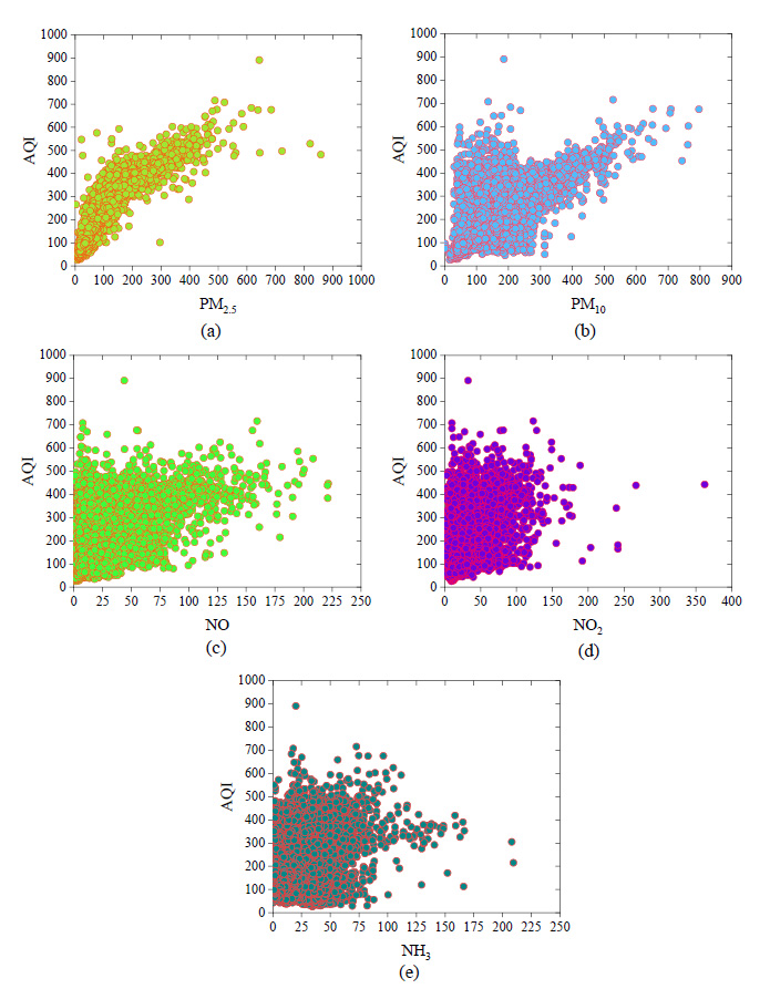
Fig. 1. Frequency distribution of input parameters (a) PM2.5; (b) PM10; (c) NO; (d) NO2; and (e) NH3.
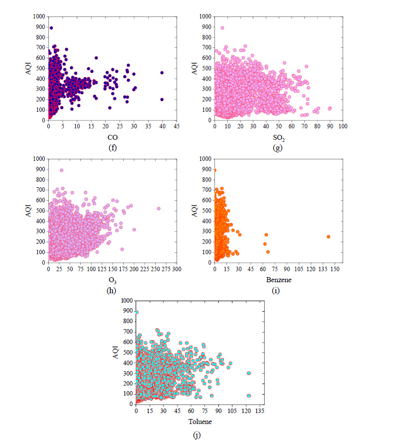
Fig. 2. Frequency distribution of input parameters (f) CO; (g) SO2; (h) O3; (i) C6H6; and (j) C7H8.
The correlation coefficient (R) values of the output and input parameters are presented in Fig. 3. The maximum value of R is in between PM2.5 and AQI and the worst correlation is found in between CO and AQI as shown in Fig. 3.
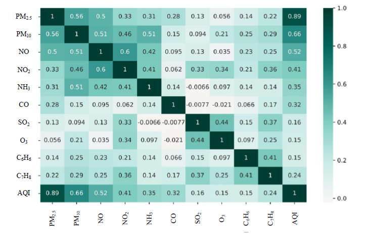
Fig. 3. Pearson’s coefficient between input and output parameters.
2.2 Performance criteria
To access the performance of neural network, the commonly used performance indicators are; coefficient of correlation (R), mean absolute error (MAE), root mean squared error (RMSE), and mean absolute percentage error (MAPE) [ 24 , 25 ] are used. R-value closes to one imply a superior association between the intended outcome, although R-values more than 0.85 show a significant correlation. The pertinent expressions of R, MAPE, MAE, and MSE are shown in Equations 1 to 4.
The methodology to achieve the current objective is shown in Fig. 4.

Fig. 4. Methodology of the present work.
Artificial intelligence
AI is a ground-breaking technology that is rapidly changing the economy, employment opportunities, and world. Social networks, internet search engines, autonomous vehicles, robot stock traders, voice assistants, etc. are some examples of common AI uses. These systems may be standalone software agents operating in the digital world or incorporated in actual mechanical devices. Because of their incredible potential to drastically alter our way of life, society and politics must comprehend and control the capabilities and restrictions of these gadgets.
The term "artificial intelligence technology" refers to the comprehensive application of cutting-edge internet and analogue computing technologies in the advancement of modern science and technology. It replicates human consciousness for fixed thinking through machine operation and develops into a form of action technology. AI is currently being used in a wide range of industries, including manufacturing, internet, and other businesses. The support of data and the support of high-power transmission technology form the basis of AI technology. It can mimic specific types of problem-solving thinking and decision-making. To accomplish the impact of quick decision-making and rapid action, a more scientific conclusion is ultimately optimized using a vast quantity of data computation [ 26 ].
3.1 Artificial neural network
ANNs have been widely employed in numerous engineering disciplines' study during the last few decades. These approaches are simple, work well, and are computationally inexpensive. The commonly used ANN is Feedforward Neural Networks (FFNN). FFNNs take information as inputs on one side and create outputs on the other side via one-way connections between neurons in multiple layers. Single and Multi-Layer Perceptrons (MLP) are the two varieties of FFNNs. In single layer perceptron (SLP), there is only one perceptron. Despite their simplicity, SLPs are unable to cope with non-linear problems. As a consequence, MLPs containing more than one perceptron are employed [ 27 ]. There are three or more layers in a multilayer perceptron (MLP), comprising input, one or more hidden layers, and one output layer. The activation function, weights, and units are all contained in the hidden layer (or neurons). The output is calculated by adding bias to the weights from the previous layer at a node and deriving the output using a transfer function. The structure of ANN for AQI prediction is shown in Fig. 4. The input layer collects information from the outside environment and sends it to hidden layer neurons without doing any computational calculations.
Prior to training the network, data standardisation was executed to eliminate unwanted feature scaling effects as well as for increasing computational stability. The Log-sigmoid activation function was used to identify values in the range -1 to 1, after all parameters were transformed linearly according to equation 5. The following is a quantitative representation of the normalizing process.
where x* = standardized value, x = measured value, xmax = highest value in the dataset, and xmin is the lowest value in data set.
3.1.1 Selection of best Neuron
The MATLAB R2021a [ 28 ] application was used to train and assess artificial neural networks (ANNs). The FFBP approach using the Levenberg-Marquardt (LM) procedure was utilised to train the suggested network in MATLAB. The usage of a single hidden layer to tackle numerous nonlinear problems has been demonstrated in the literature. Throughout this layer-by-layer training procedure, the input signals were transmitted forward and the error signals were returned. The weights were adjusted until the output layer produced the anticipated result. On a random basis, 6617 dataset points were separated into three categories. A total of 4632 data (70%), 993 data (15%), and 993 data (15%) were collected for training, validation, and testing, sequentially. The training and validation sets were utilized in the network training process, and performance of the networks were evaluated using the testing and training datasets.
The optimal number of neurons and the appropriate ANN were discovered through trial and error procedures. The optimal ANN design was defined in this study using 3 to 12 number of neurons. Conventional statistical errors and performance indicators, such as MSE and R, were used to select the best network architecture. As a consequence, each pattern's evaluation index is calculated, and the results are established based on the replies' competency. Finally, compute the rank for each of the proposed patterns, and choose the network's best design. Table 3 shows the results of the artificial neural network's AQI assessment.
| Neuron | Values | Rank | Total | ||||||||
|---|---|---|---|---|---|---|---|---|---|---|---|
| R | MSE | R | MSE | ||||||||
| Tr. | Val. | Te. | All | Tr | Val | Te | All | All | All | ||
| 3 | 0.9569 | 0.9588 | 0.9444 | 0.9533 | 0.0066 | 0.0059 | 0.0087 | 0.0071 | 10 | 9 | 19 |
| 4 | 0.9500 | 0.9432 | 0.9526 | 0.9486 | 0.0079 | 0.0087 | 0.0073 | 0.0080 | 9 | 10 | 19 |
| 5 | 0.9596 | 0.9604 | 0.9502 | 0.9567 | 0.0061 | 0.0063 | 0.0076 | 0.0067 | 6 | 6 | 12 |
| 6 | 0.9602 | 0.9544 | 0.9529 | 0.9558 | 0.0059 | 0.0070 | 0.0077 | 0.0069 | 7 | 7 | 14 |
| 7 | 0.9612 | 0.9502 | 0.9594 | 0.9569 | 0.0058 | 0.0075 | 0.0064 | 0.0066 | 5 | 5 | 10 |
| 8 | 0.9585 | 0.9571 | 0.9659 | 0.9605 | 0.0063 | 0.0064 | 0.0051 | 0.0060 | 2 | 2 | 4 |
| 9 | 0.9611 | 0.9643 | 0.9591 | 0.9615 | 0.0059 | 0.0052 | 0.0066 | 0.0059 | 1 | 1 | 2 |
| 10 | 0.9634 | 0.9533 | 0.9444 | 0.9537 | 0.0056 | 0.0072 | 0.0083 | 0.0070 | 8 | 8 | 16 |
| 11 | 0.9627 | 0.9630 | 0.9497 | 0.9585 | 0.0057 | 0.0058 | 0.0074 | 0.0063 | 3 | 3 | 6 |
| 12 | 0.9625 | 0.9621 | 0.9490 | 0.9579 | 0.0057 | 0.0059 | 0.0079 | 0.0065 | 4 | 4 | 8 |
According to the ranking algorithms, the 9 neurons were recognized as the best network out of all of the neurons in Table 3. The chosen neural estimating networks are shown in schematic form in Fig. 6. In the chosen network for testing, training and validation analysis, R and MSE are 0.9643, 0.9611, and 0.9591, respectively, with remarkably tiny values of 0.0052, 0.0066 and 0.0059, respectively.
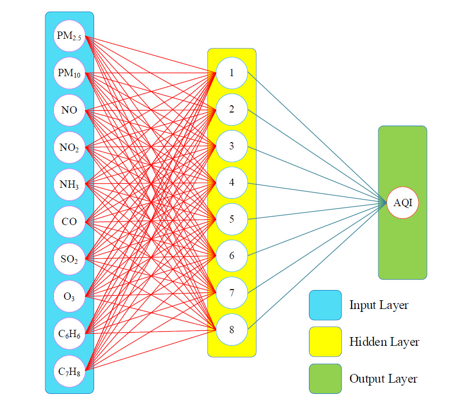
Fig. 5. Structure of ANN.
3.2 Gaussian process regression
Gaussian processes regression was also used to calculate the predictions for the air quality. A supervised learning approach, the GP regression method [ 29 ] is used. The ability to get a predicted mean and a predictive variance using GP regression is one advantage of using it to estimate quality of air. Both the mean function and the covariance function of the Gaussian process fully describe in [ 29 ]. It is also known as the function-space view.
The Gaussian assumption and the marginalization feature of the Gaussian process, which presupposes that the joint distribution is Gaussian, may be used to derive the predictive distribution from this. 10-fold cross-validation process was used to validate the results of GPR model.Regression using Gaussian processes necessitates choosing a covariance function. A approach to incorporate past knowledge of the phenomenon into the study is through the covariance function and certain of its parameters. Equation 9 shows the so-called squared exponential covariance function is used in this study. The stationary squared exponential covariance function's structure puts a focus on nearby locations. Thus, the local behaviour of a smooth function is comparable.
where, l is the characteristics length-scale.
4. Results and discussion
Auto Regressive Integrate Moving Average (ARIMA) as a time series model, Principal Component Regression (PCR) as a hybrid regression model, combination of ARIMA and PCR as the first ensemble model and, the combination of ARIMA and Gene Expression Programming (GEP) as the second ensemble model. Observed AQI during the years 2012 to 2015 was utilized to train models. According to the results, nonlinear ensemble model is considered as the best model for predicting AQI in all seasons. The maximum negative and positive errors, Mean Absolute Percentage Error (MAPE), and statistical parameters, including the coefficient of determination, root mean square error (RMSE), normalized square error (NMSE), and fractional bias, were utilized to evaluate and compare models [ 35 ].These models are autoregressive conditional heteroscedasticity (GARCH), autoregressive integrated moving average (ARIMA), and the combination of ARIMA and GARCH by multiple linear regression (MLR) technique (model 3). Correlation coefficient, root mean square error (RMSE), normalized square error (NMSE), and fractional bias, are calculated to evaluate the accuracy of each model. ARIMA and model 3 can predict future earthquake magnitude better than other models [ 10 ].The neuron in the ANN algorithm has been studied from 3 to 12 number. To quantify the performance of each ANN model at each individual neuron, the performance indices R and MSE for training, testing, and validation datasets are utilized. According to Table 3, neuron 9 has the greatest R value and the lowest MSE value, as well as the lowest rank among all the neurons, as presented in Table 3. The R, RMSE, MAPE, and MAE values of the ANN model is 0.9611, 33.2762, 13.2468, and 22.9362, respectively. The values of the performance indices for training, testing, validation and all dataset in is shown in Table 4. Fig. 6 shows the scatter plot between the measured AQI and the predicted AQI values for training, testing, validation and all dataset. On the right side of the scatter plot, a line diagram shows the measured and predicted value respect to errors. The error range for the training, testing, validation and all dataset are -289.44 to 456.99, -171.83 to 139.58, -99.83 to 171.46 and -284.44 to 456.99, respectively.The results of the GPR model is shown in last column of Table 4. The overall performance of GPR model in terms of R, RMSE, MAPE and MAE are 0.9843, 21.41, 10.04 and 13.59, respectively. Fig. 7 shows the plot between the measure and predicted AQI with respected the errors. The error range in the GPR model for training, testing and all dataset are -102.87 to 259.64, -174.19 to 328.11 and -174.19 to 328.11, respectively.
| ANN | GPR | ||
|---|---|---|---|
| Performance Indices | Values | ||
| R | Training | 0.9589 | 0.9923 |
| Testing | 0.9508 | 0.9653 | |
| Validation | 0.9673 | - | |
| All | 0.9611 | 0.9843 | |
| RMSE | Training | 31.1999 | 15.0281 |
| Testing | 31.7113 | 31.6395 | |
| Validation | 30.2592 | - | |
| All | 33.2762 | 21.40797 | |
| MAPE | Training | 13.2114 | 5.8660 |
| Testing | 13.3076 | 12.6279 | |
| Validation | 13.3521 | - | |
| All | 13.2468 | 7.8945 | |
| MAE | Training | 23.0929 | 10.0413 |
| Testing | 22.702 | 21.8658 | |
| Validation | 22.4394 | - | |
| All | 22.9362 | 13.5884 | |
| Model | R | RMSE | MAPE | MAE |
|---|---|---|---|---|
| ANN | 0.9611 | 33.2762 | 13.2468 | 22.9362 |
| GPR | 0.9843 | 21.4079 | 7.8945 | 13.5884 |
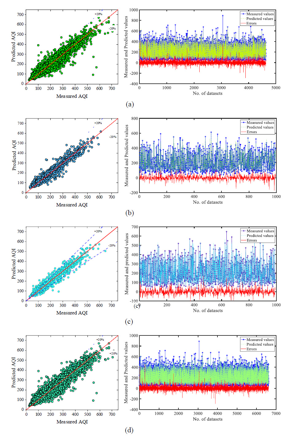
Fig. 6. ANN (a) Training dataset, (b) Testing dataset, (c) Validation dataset and (d) All dataset.
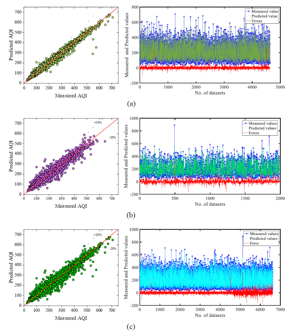
Fig. 7. GPR (a) Training dataset, (b) Testing dataset, and (c) All dataset.
Taylor diagram is plotted in between the correlation coefficient, standard deviation and RMSE. Fig. 8 shows the graphical representation of the performance of the ANN and GPR model. Dotted green line in the Fig. 8 is the “reference” line based on the measured value of the dataset. Based on the performance indices and the Taylor diagram it is concluded that the performance of the GPR model is higher as compared to ANN model.
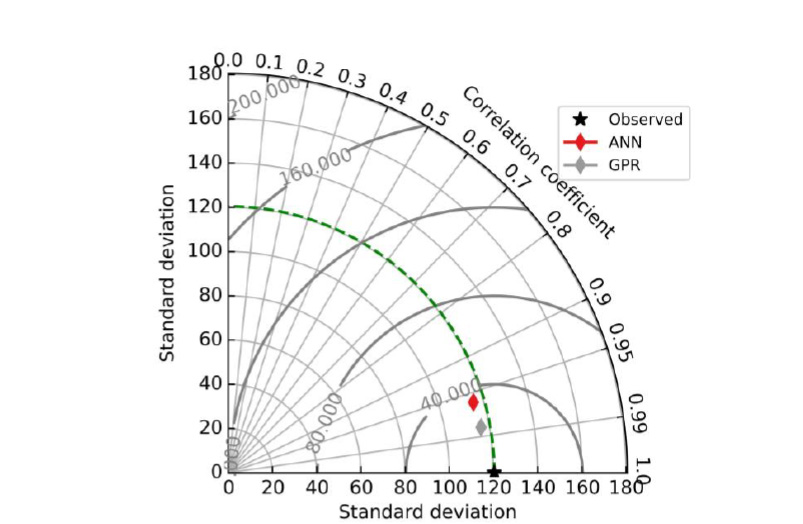
Fig. 8. Graphical representation of the model using Taylor Plot.
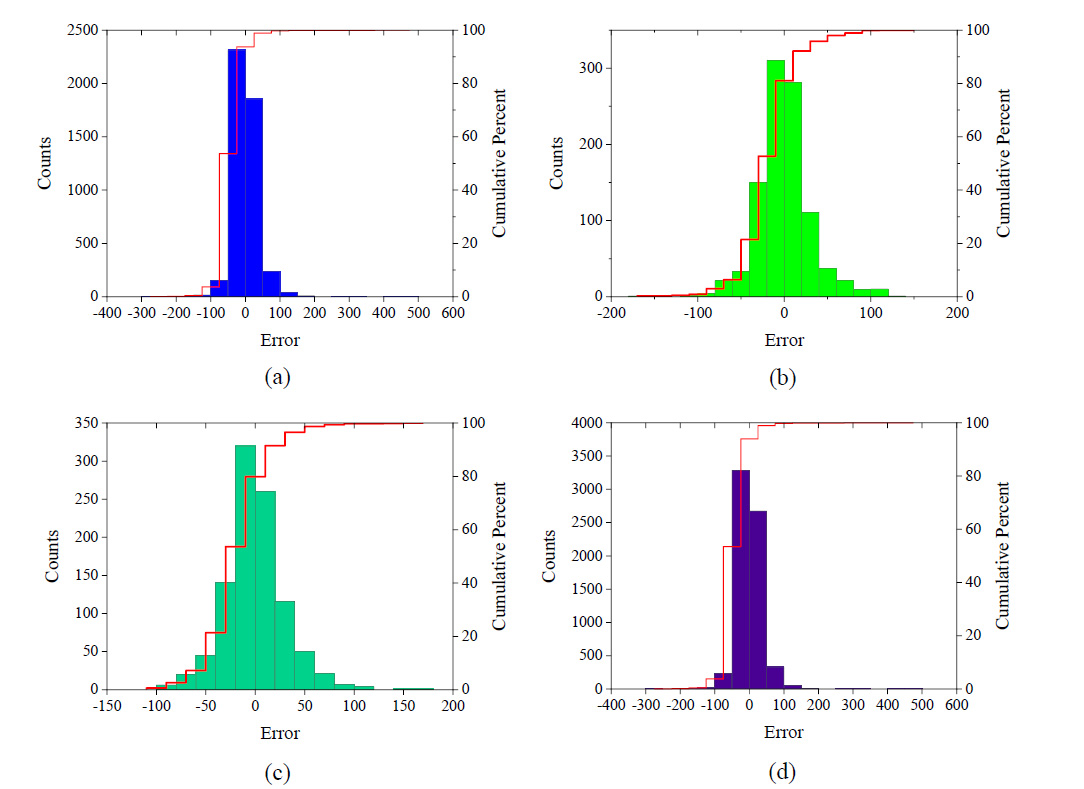
Fig. 9. Error Frequency histogram of ANN Model (a) Training dataset, (b) Testing dataset, (c) Validation dataset and (d) All dataset.
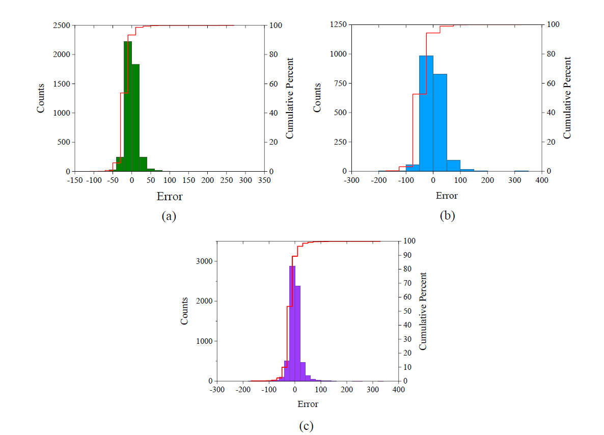
Fig. 10. Error frequency histogram of GPR model (a) Training dataset (b) Testing dataset and (c) All dataset.
Error Frequency histogram of GPR Model (a) Training data, (b) Testing data and (c) All dataset
The proposed formulation to predict the AQI is expressed in equation:
The values of G1, G2 …., and G8 is mentioned in equation
In summary, three single models, including a Step-By-Step Regression (SBSR), Gene Expression Programming (GEP), and an Adaptive Neuro-Fuzzy Inference System (ANFIS) as well as three hybrid models, i.e. HCVCM-SBSR, HCVCM-GEP, and HCVCM-ANFIS are employed to predict the compressive strength of concrete. The statistical parameters and error terms such as the coefficient of determination, the Root Mean Square Error (RMSE), Normalized Mean Square Error (NMSE), fractional bias, the maximum positive and negative errors, and the Mean Absolute Percentage Error (MAPE) are computed to evaluate the models. The results show that HCVCM-ANFIS can predict the compressive strength of concrete better than all other models [ 30 ]. Moreover, five prediction models, including step-by-step regression (SBSR), the combination of stronger variable creator machine (SVCM) and SBSR, gene expression programming (GEP), the combination of SVCM and GEP, and adaptive neuro-fuzzy inference system (ANFIS), were utilized to predict the compressive and flexural strengths of the stones. All models were compared using statistical parameters and error terms. ANFIS performs better than all other models [ 31 ].
5. Conclusion and limitation of the work
In this study, the AQI model is developed, on the basis of ten different gases such as PM2.5, PM, NO, NO2. AOI may be predicted using a numerical technique based on the ML algorithms. The ANN and GPR model are built using 6617 datasets and considering PM2.5, PM10, NO, NO2, NH3, CO, SO2, O3, C6H6, and C7H8 as the inputs. The following are the paper's primary conclusions:
- The suggested ANN model appears to be a viable tool for extracting features and forecasting inexpressible situations with numerous influence factors. The ANN architecture must be tuned by trial and error calculations based on the dataset's size and complexity. The amount and quality of the dataset used determines the ANN model's efficacy and accuracy.
- The correlation coefficient of ANN and GPR models are 0.9611 and 0.9843, sequentially. The values of RMSE, MAPE and MAE of the ANN model are 33.28, 13.24% and 22.94, respectively.
- The performance of the indices of the GPR model are 21.41, 7.89% and 13.59 for RMSE, MAPE and MAE, respectively.
- The suggested equation based on the ANN and built networks can account for the effects of C6H6 and C7H8 on the air quality index.
- The analysed results shows that the precision and reliability of the GPR model is superior as compared to ANN model.
- The proposed network and equation can only able to predict the AQI that falls within the range of input parameters.
Funding
This research received no external funding.
Conflicts of interest
The authors declare no conflict of interest.
Authors contribution statement
Raunaq Singh Suri: Conceptualization, Data curation, Methodology, Original draft, Writing - review & editing; Ajay Kumar Jain: Formal analysis, Investigation, Methodology; Nishant Raj Kapoor: Data curation, Writing - review & editing; Aman Kumar: Visualization, Software, Harish Chandra Arora: Resources, Writing - review & editing; Krishna Kumar: Software, Writing - review & editing; Hashem Jahangir: Project administration, Visualization, Writing - review & editing.
References
- Ten threats to global health in 2019 2019. https://www.who.int/news-room/spotlight/ten-threats-to-global-health-in-2019.Publisher Full Text
- Murray CJL, Aravkin AY, Zheng P, Abbafati C, Abbas KM, Abbasi-Kangevari M, et al. Global burden of 87 risk factors in 204 countries and territories, 1990-2019: a systematic analysis for the Global Burden of Disease Study 2019. The Lancet. 2020; 396:1223-49. http://doi.org/10.1016/S0140-6736(20)30752-2. Publisher Full Text
- Lee B-J, Kim B, Lee K. Air Pollution Exposure and Cardiovascular Disease. Toxicological Research. 2014; 30:71-5. http://doi.org/10.5487/TR.2014.30.2.071. Publisher Full Text
- Apte JS, Brauer M, Cohen AJ, Ezzati M, Pope CA. Ambient PM 2.5 Reduces Global and Regional Life Expectancy. Environmental Science & Technology Letters. 2018; 5:546-51. http://doi.org/10.1021/acs.estlett.8b00360. Publisher Full Text
- Wong EY, Gohlke J, Griffith WC, Farrow S, Faustman EM. Assessing the health benefits of air pollution reduction for children. Environmental Health Perspectives. 2004; 112:226-32. http://doi.org/10.1289/ehp.6299. Publisher Full Text
- Cao L, Zhai D, Kuang M, Xia Y. Indoor air pollution and frailty: A cross-sectional and follow-up study among older Chinese adults. Environmental Research. 2022; 204:112006. http://doi.org/10.1016/j.envres.2021.112006. Publisher Full Text
- Agarwal N, Meena CS, Raj BP, Saini L, Kumar A, Gopalakrishnan N, et al. Indoor air quality improvement in COVID-19 pandemic: Review. Sustainable Cities and Society. 2021; 70:102942. http://doi.org/10.1016/j.scs.2021.102942. Publisher Full Text
- Pi T, Wu H, Li X. Does Air Pollution Affect Health and Medical Insurance Cost in the Elderly: An Empirical Evidence from China. Sustainability. 2019; 11:1526. http://doi.org/10.3390/su11061526. Publisher Full Text
- Power AL, Tennant RK, Jones RT, Tang Y, Du J, Worsley AT, et al. Monitoring Impacts of Urbanisation and Industrialisation on Air Quality in the Anthropocene Using Urban Pond Sediments. Frontiers in Earth Science. 2018; 6. http://doi.org/10.3389/feart.2018.00131Publisher Full Text
- Mo, Zhang, Li, Qu. A Novel Air Quality Early-Warning System Based on Artificial Intelligence. International Journal of Environmental Research and Public Health. 2019; 16:3505. http://doi.org/10.3390/ijerph16193505. Publisher Full Text
- Bai L, Wang J, Ma X, Lu H. Air Pollution Forecasts: An Overview. International Journal of Environmental Research and Public Health. 2018; 15:780. http://doi.org/10.3390/ijerph15040780. Publisher Full Text
- Jerrett M, Arain A, Kanaroglou P, Beckerman B, Potoglou D, Sahsuvaroglu T, et al. A review and evaluation of intraurban air pollution exposure models. Journal of Exposure Science & Environmental Epidemiology. 2005; 15:185-204. http://doi.org/10.1038/sj.jea.7500388. Publisher Full Text
- Rahimi A. Short-term prediction of NO2 and NO x concentrations using multilayer perceptron neural network: a case study of Tabriz, Iran. Ecological Processes. 2017; 6:4. http://doi.org/10.1186/s13717-016-0069-x. Publisher Full Text
- Karatzas KD, Kaltsatos S. Air pollution modelling with the aid of computational intelligence methods in Thessaloniki, Greece. Simulation Modelling Practice and Theory. 2007; 15:1310-9. http://doi.org/10.1016/j.simpat.2007.09.005. Publisher Full Text
- Chaloulakou A, Saisana M, Spyrellis N. Comparative assessment of neural networks and regression models for forecasting summertime ozone in Athens. Science of The Total Environment. 2003; 313:1-13. http://doi.org/10.1016/S0048-9697(03)00335-8. Publisher Full Text
- Mishra D, Goyal P, Upadhyay A. Artificial intelligence based approach to forecast PM 2.5 during haze episodes: A case study of Delhi, India. Atmospheric Environment. 2015; 102:239-48. http://doi.org/10.1016/j.atmosenv.2014.11.050. Publisher Full Text
- Freeman BS, Taylor G, Gharabaghi B, Thé J. Forecasting air quality time series using deep learning. Journal of the Air & Waste Management Association. 2018; 68:866-86. http://doi.org/10.1080/10962247.2018.1459956. Publisher Full Text
- Soh P-W, Chang J-W, Huang J-W. Adaptive Deep Learning-Based Air Quality Prediction Model Using the Most Relevant Spatial-Temporal Relations. IEEE Access. 2018; 6:38186-99. http://doi.org/10.1109/ACCESS.2018.2849820. Publisher Full Text
- Qi Y, Li Q, Karimian H, Liu D. A hybrid model for spatiotemporal forecasting of PM2.5 based on graph convolutional neural network and long short-term memory. Science of The Total Environment. 2019; 664:1-10. http://doi.org/10.1016/j.scitotenv.2019.01.333. Publisher Full Text
- Kumar K, Pande BP. Air pollution prediction with machine learning: a case study of Indian cities. International Journal of Environmental Science and Technology. 2022. http://doi.org/10.1007/s13762-022-04241-5. Publisher Full Text
- Van NH, Van Thanh P, Tran DN, Tran D-T. A new model of air quality prediction using lightweight machine learning. International Journal of Environmental Science and Technology. 2022. http://doi.org/10.1007/s13762-022-04185-w. Publisher Full Text
- Shishegaran A, Saeedi M, Kumar A, Ghiasinejad H. Prediction of air quality in Tehran by developing the nonlinear ensemble model. Journal of Cleaner Production. 2020; 259:120825. http://doi.org/10.1016/j.jclepro.2020.120825. Publisher Full Text
- Air Quality Data in India (2015 - 2020) 2020. https://www.kaggle.com/datasets/rohanrao/air-quality-data-in-india (accessed December 28, 2022).Publisher Full Text
- Fakharian P, Rezazadeh Eidgahee D, Akbari M, Jahangir H, Ali Taeb A. Compressive strength prediction of hollow concrete masonry blocks using artificial intelligence algorithms. Structures. 2023; 47:1790-802. http://doi.org/10.1016/j.istruc.2022.12.007. Publisher Full Text
- Rezazadeh Eidgahee D, Jahangir H, Solatifar N, Fakharian P, Rezaeemanesh M. Data-driven estimation models of asphalt mixtures dynamic modulus using ANN, GP and combinatorial GMDH approaches. Neural Computing and Applications. 2022. http://doi.org/10.1007/s00521-022-07382-3. Publisher Full Text
- Shi T, Wu J. Application of Artificial Intelligence in Water Conservancy Project Management. 2021 2nd International Conference on Big Data & Artificial Intelligence & Software Engineering (ICBASE), IEEE; 2021, p. 556-9. http://doi.org/10.1109/ICBASE53849.2021.00109.Publisher Full Text
- Jahangir H, Rezazadeh Eidgahee D. A new and robust hybrid artificial bee colony algorithm - ANN model for FRP-concrete bond strength evaluation. Composite Structures. 2021; 257:113160. http://doi.org/10.1016/j.compstruct.2020.113160. Publisher Full Text
- Demuth H, Beale M. Matlab neural network toolbox user’s guide version 6. 2009.
- Caywood MS, Roberts DM, Colombe JB, Greenwald HS, Weiland MZ. Gaussian Process Regression for Predictive But Interpretable Machine Learning Models: An Example of Predicting Mental Workload across Tasks. Frontiers in Human Neuroscience. 2017; 10. http://doi.org/10.3389/fnhum.2016.00647Publisher Full Text
- Shishegaran A, Varaee H, Rabczuk T, Shishegaran G. High correlated variables creator machine: Prediction of the compressive strength of concrete. Computers & Structures. 2021; 247:106479. http://doi.org/10.1016/j.compstruc.2021.106479. Publisher Full Text
- Shishegaran A, Saeedi M, Mirvalad S, Korayem AH. Computational predictions for estimating the performance of flexural and compressive strength of epoxy resin-based artificial stones. Engineering with Computers. 2022. http://doi.org/10.1007/s00366-021-01560-y. Publisher Full Text
